The oscillating dipole

In 2015, I submitted my Part III (Master's) project at Cambridge under the supervision of Steve Gull. The project was titled Animation of Electric and Magnetic Field Lines and covered a range of problems: the method of images, rotating conductors in magnetic fields, relativistic charges, and the oscillating electric dipole. All visualised in MATLAB.

A decade later, I wanted to revisit the part I found most beautiful: the electric dipole and how its field lines reveal the mechanism of radiation. This time, the visualisations run in your browser.

The static dipole

An electric field line is the path a tiny positive test charge would follow if you released it into the field. At every point along the curve, the line is tangent to the electric field, showing you the direction the field would push a charge.

Field lines are a visualisation tool, not physical objects. You can't see an electric field. You can only measure the force it exerts on a charge. The field line picture is a global construct: it connects the electric field at every point in space into coherent curves at a single instant in time. No observer experiences this. A test charge sitting far from the dipole feels the field oscillating up and down, a local periodic force. It has no concept of being "on a field line" or of a loop sweeping past.

When we later watch field lines "detach" and "propagate outward," the electric field at each point in space is oscillating, and the pattern of contours shifts outward over time. A wave on water is a moving shape, not moving water. The detaching loops work the same way: an artifact of how we choose to draw contours of a global function, not something a local observer would see.

But the radiation is real. It carries energy and momentum. If you place an antenna (a conductor with mobile charges) in the path of an outgoing wave, the oscillating electric field pushes charges back and forth inside it. That's radio reception. The field lines are a map; the territory is forces on charges.

The electric dipole is the simplest interesting charge distribution: two equal and opposite charges $+q$ and $-q$, separated by a small distance $d$ along the $z$-axis.

Let's derive the field from scratch. Place $+q$ at $z = +d/2$ and $-q$ at $z = -d/2$. A single point charge $q$ produces a Coulomb potential $\phi = q / (4\pi\epsilon_0 r)$, so the total potential at a point $\mathbf{r}$ is

where $r_+$ and $r_-$ are the distances from $\mathbf{r}$ to the positive and negative charges. When we're far from the dipole ($r \gg d$), these distances are approximately

where $\theta$ is the angle from the $z$-axis. Using $1/(r - \epsilon) \approx 1/r + \epsilon/r^2$ for small $\epsilon$:

The $1/r$ terms cancel (the charges are equal and opposite), and what survives is:

where $p = qd$ is the dipole moment. The potential falls off as $1/r^2$, one power faster than a single charge, because the two Coulomb potentials almost cancel.

The electric field is $\mathbf{E} = -\nabla\phi$. Taking the gradient in spherical coordinates:

So the electric field of the dipole is

This is a $1/r^3$ field. The cancellation between the two charges has cost us a power of $r$. The $\cos\theta$ term points radially (strong on-axis), the $\sin\theta$ term curves around in the $\hat{\boldsymbol\theta}$ direction (strong at the equator). Together they produce the classic pattern:

Field lines emerge from the positive pole (top), arc outward, and return to the negative pole (bottom). Along the axis they're tightly packed; in the equatorial plane they spread out. The pattern is static. No energy leaves. The field sits there.

Field lines and the stream function

The brute-force way to draw field lines is to pick a starting point, evaluate $\mathbf{E}$ there, take a small step in the direction of $\mathbf{E}$, evaluate again, step again, tracing out the curve numerically. In differential equation form, you're solving

where $s$ is the arc length along the field line. This works, but it's slow (you need many steps per line), sensitive to step size near singularities, and the starting points need to be chosen with care to get an even distribution of lines.

For problems with azimuthal symmetry (the field looks the same from every angle around the $z$-axis), there's a better approach.

The idea starts with a fact from multivariable calculus: the contour lines of a scalar function are always perpendicular to its gradient. Think of a topographic map: the contour lines (constant elevation) run perpendicular to the direction of steepest ascent. So if we can find a scalar function $\Psi$ whose gradient is perpendicular to the electric field at every point, then the contour lines of $\Psi$ are the field lines. No differential equations, no numerical integration. A contour plot.

How do you find such a $\Psi$? For a divergence-free field with azimuthal symmetry, the electric field can be written as $\mathbf{E} = \nabla \times \mathbf{G}$ for some vector field $\mathbf{G} = G_\phi\,\hat{\boldsymbol\phi}$. Expanding the curl in cylindrical coordinates $(\rho, \phi, z)$:

Now compute $\mathbf{E} \cdot \nabla(\rho G_\phi)$. The two terms cancel: the field is perpendicular to the gradient of $\rho G_\phi$. So define $\Psi = \rho G_\phi$, and we have our scalar function. Its contour lines are the field lines.

For the static dipole, $\Psi = \sin^2\theta / r$. The visualisation above is a contour plot of this function.

The oscillating dipole

Now let the dipole moment oscillate: $\mathbf{p}(t) = p_0\cos(\omega t)\,\hat{\mathbf{z}}$. This is the Hertz dipole, the simplest source of electromagnetic radiation.

The wavenumber $k = \omega / c = 2\pi / \lambda$ (where $\lambda$ is the wavelength) controls how much the dipole radiates. The wavenumber is inversely proportional to wavelength: small $k$ means a long wavelength (the field changes slowly in space and barely radiates), while large $k$ means a short wavelength (the field oscillates rapidly and radiates aggressively). Think of $k$ as a dial between "static" and "radiating."

When the dipole oscillates, changes in the field propagate outward at the speed of light, not instantaneously. The full electric field (derived from retarded potentials, which account for this finite propagation speed) has three terms, each dominating at a different distance from the source.

The near field ($kr \ll 1$, close to the source):

This is the static dipole field, oscillating in sync with the source. It falls off as $1/r^3$: strong nearby, negligible far away. It carries no energy outward.

The intermediate field ($kr \sim 1$):

This $1/r^2$ term bridges the near and far regions. The field lines start to distort and bulge outward.

The radiation field ($kr \gg 1$, far from the source):

This is the term that matters. It falls off as $1/r$. The energy it carries (proportional to $E^2 \sim 1/r^2$), integrated over a sphere of radius $r$ (area $\sim r^2$), gives a constant. Energy escapes to infinity.

The radiation term points in the $\hat{\boldsymbol\theta}$ direction (transverse to propagation), like a transverse electromagnetic wave. It vanishes on the axis ($\sin\theta = 0$): the dipole doesn't radiate along its axis, only in the equatorial directions.

The stream function trick still works. The combined field can be written as a curl, and the stream function becomes:

The first term (decaying as $1/r$) is the near field; the second (constant amplitude $k$) is the radiation field. Contour lines of $\Psi$ are the field lines, now animated:

Use the slider to change $k$. At $k = 0$ you recover the static dipole. As you increase $k$, watch what happens: field lines near the dipole still oscillate back and forth, but further out, loops pinch off and radiate outward. You're watching electromagnetic radiation form.

The physics of field line detachment

The boundary between near field and radiation is where the action is. Watch the animation. Information travels at a finite speed.

When the dipole reverses direction (say, from pointing up to pointing down), the reversal takes time to propagate. The new field configuration propagates outward at the speed of light. But the old field, the one from the previous half-cycle, is still out there, propagating away. For a brief moment, there's a boundary at roughly $r \sim 1/k = \lambda / (2\pi)$ where the outgoing field from the old half-cycle meets the reversing near-field from the new one. These fields point in opposite directions. They cancel.

At this cancellation surface, the field strength drops to zero. The field lines reconnect: what was a continuous arc from pole to pole pinches shut at the equator. The outer portion forms a closed loop, now disconnected from the source. This loop propagates outward at the speed of light, never to return.

In each half-cycle:

1. New field lines emerge from the dipole
2. They expand outward
3. At $r \sim \lambda / (2\pi)$, the old outgoing field and the new reversed field cancel
4. The field lines pinch together at the equator, reconnect, and form a closed loop
5. The detached loop propagates outward as radiation

These escaping closed loops of electric field are the radiation. They carry energy away from the dipole. The power radiated is proportional to $\omega^4$ (or equivalently $k^4$), the Larmor formula result. Higher frequency means far more radiation.

Why the sky is blue

The $\omega^4$ dependence has a beautiful consequence. When sunlight hits the atmosphere, it drives the electrons in air molecules into oscillation. Each molecule becomes a tiny oscillating dipole, re-radiating the light in all directions. This is Rayleigh scattering.

But the re-radiation efficiency goes as $\omega^4$. Blue light ($\lambda \approx 450$ nm) has a wavelength about 1.8 times shorter than red light ($\lambda \approx 700$ nm), so its frequency is 1.8 times higher. The radiated power scales as $\omega^4$, so blue scatters $(1.8)^4 \approx 5.4$ times more than red. The sky is blue. Sunsets are red because you're looking through so much atmosphere that the blue has been scattered away, leaving the red.

The oscillating dipole is the mechanism behind the colour of the sky.

AM radio: modulating the dipole

The oscillating dipole above radiates at a single frequency, a pure carrier wave. But a pure sine wave carries no information. To transmit a voice or music, you need to modulate the carrier: vary one of its properties (amplitude, frequency, or phase) in proportion to the signal you want to send.

Hit play to hear the most famous radio transmission in history: Neil Armstrong's words from the Moon, relayed to Earth via AM radio on July 20, 1969.

The top panel shows the full waveform. The middle panel zooms into a 50 ms window around the playhead, enough to see the oscillations of Armstrong's voice. The bottom panel zooms again to 2 ms, where you can see individual samples: the discrete measurements that a digital system stores. This recording has 44,100 of them per second.

AM (amplitude modulation) is the simplest modulation scheme. The transmitted signal is

where $a(t)$ is the audio signal (normalised to $[-1, 1]$), $\omega_c$ is the carrier frequency, and $m \in [0, 1]$ is the modulation depth, how much the audio swings the carrier's amplitude. At $m = 0$, the carrier is unmodulated. At $m = 1$, the carrier's amplitude swings from zero to twice its resting value.

In terms of our dipole, the carrier is the oscillating dipole moment $p_0\cos(\omega_c t)$. Amplitude modulation replaces $p_0$ with $p_0[1 + m\,a(t)]$: the dipole oscillates harder when the audio signal is loud and softer when it's quiet. The radiation pattern is still that of a Hertzian dipole; only the envelope changes.

A receiver extracts the audio by demodulating: rectifying the signal (removing the negative half-cycles) and low-pass filtering to recover the envelope. The signal arriving at the antenna is the radiation field of the transmitting dipole, attenuated by the $1/r$ falloff we derived earlier. The AM broadcast band (530–1700 kHz) uses wavelengths of 175–565 metres, far larger than any practical antenna, so the stations all operate in the Hertzian dipole regime.

The computation

The stream function is

and the field lines are its contours. So the computational problem is: evaluate $\Psi$ on a grid, find contour lines, repeat every frame.

Separating space and time

The key trick is expanding the time dependence. Since $\cos(kr - \omega t) = \cos(kr)\cos(\omega t) + \sin(kr)\sin(\omega t)$ (and similarly for $\sin$), we can split $\Psi$ into two purely spatial functions:

Then each frame is

We precompute $A$ and $B$ once (they only change when $k$ changes), and each frame becomes a cheap weighted sum over the grid. Setting $c = \omega = 1$ keeps things simple.

Coordinate mapping

We work on a square grid of pixels, mapped to physical coordinates $(\rho, z)$ over some range. At each grid point:

There's a singularity at the origin where $r = 0$. We mask it out (any point with $r < 0.15$ is skipped) and draw a dot there instead.

Finding contour lines

Given $\Psi$ on the grid, we need to find curves where $\Psi = c$ for a set of contour values. The CPU version does this by brute force: for each pixel, for each contour value $c$, check whether $\Psi - c$ changes sign between neighbouring pixels. If it does, a contour line passes through that pixel, and we colour it dark.

The contour values are geometrically spaced: $c_n = 0.01 \times 1.45^n$, with both positive and negative values. This gives good coverage: dense near $\Psi = 0$ (where lines are tightly packed) and sparse at large $|\Psi|$. About 20 contour values total, checked at every pixel, every frame.

The original MATLAB code from 2015 did the same thing, but I like that this runs interactively in a browser a decade later.

CPU vs GPU

The CPU version has an obvious bottleneck: the contour detection. Each frame, for each of ~2 million pixels, it checks ~20 contour values for sign changes against two neighbours. That's tens of millions of comparisons per frame, all single-threaded. The precomputed $A$/$B$ trick saves us from recomputing the trig every frame, but the contour scan is still expensive.

The same computation maps well onto a GPU. Each pixel is independent: the stream function $\Psi(\rho, z, t)$ depends on the pixel's coordinates and the current time. Fragment shaders do this: run the same small program on every pixel in parallel.

The WebGL version below computes everything in a single GLSL fragment shader. The physics is identical, but the contour rendering is different.

Contours in log space

The CPU version checks each contour value one by one. But our contour values are geometrically spaced: $c_n = 0.01 \times 1.45^n$. Taking logarithms:

In log space, these are evenly spaced, with spacing $\log 1.45$. So the shader transforms $|\Psi|$ into this log space:

Now the contour values sit at integer values of $\ell$. To find whether the current pixel is near a contour, check how close $\ell$ is to the nearest integer, which is fract. One computation replaces twenty.

For anti-aliasing, the shader uses fwidth(l), which gives the screen-space rate of change of $\ell$. When a contour line is one pixel wide, fwidth tells the shader how to blend the line edge via smoothstep. Where contours pack tighter than a pixel (large fwidth), the lines fade out instead of creating moiré patterns.

No precomputation needed

The shader doesn't bother with the $A$/$B$ grid trick. The GPU evaluates $\Psi = A\cos(\omega t) + B\sin(\omega t)$ from scratch every frame, for every pixel, and it's still effortless. The precomputed spatial grids that saved the CPU from redundant trig are unnecessary when you have thousands of cores.

The result looks different (the lines are smoother, the contour spacing not identical) but the physics is the same.

Hertz's drawings

Heinrich Hertz drew these field line patterns by hand in 1889, two years after his experimental confirmation of electromagnetic waves. His drawings in Electric Waves are accurate, produced without any computational aid.

Previous slideNext slide

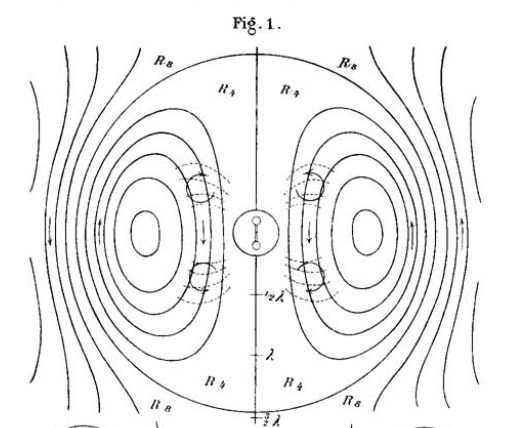
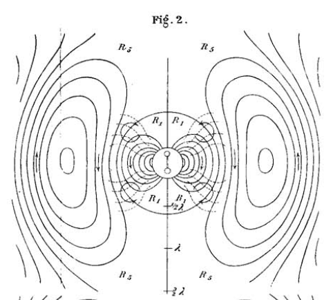
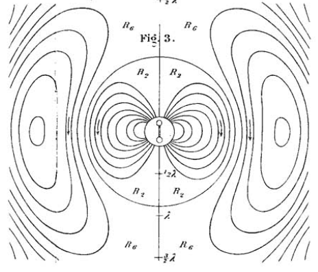
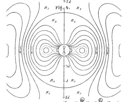
The same patterns that took him painstaking manual construction can now be computed at 60 frames per second in a few hundred lines of JavaScript.

Revisiting this problem a decade later, I'm struck by how much the visualisations reveal that the equations hide. The three-term decomposition of the electric field (near, intermediate, radiation) is clean on paper, but it doesn't prepare you for the moment you watch a field line pinch shut and a closed loop escape at the speed of light. The equations say radiation carries energy to infinity. The animation shows you how: a repeating act of topological surgery, the field tearing free from the source that created it.